Programming with Python

Analyzing Patient Data

Words are useful, but what’s more useful are the sentences and stories we build with them. Similarly, while a lot of powerful, general tools are built into languages like Python, specialized tools built up from these basic units live in libraries that can be called upon when needed.

In order to load our inflammation data, we need to import a library called NumPy. In general you should use this library if you want to do fancy things with numbers, especially if you have matrices or arrays. We can load NumPy using:

import numpy

Importing a library is like getting a piece of lab equipment out of a storage locker and setting it up on the bench. Libraries provide additional functionality to the basic Python package, much like a new piece of equipment adds functionality to a lab space. Once you’ve loaded the library, we can ask the library to read our data file for us:

numpy.loadtxt(fname='inflammation-01.csv', delimiter=',')

array([[ 0.,  0.,  1., ...,  3.,  0.,  0.],
       [ 0.,  1.,  2., ...,  1.,  0.,  1.],
       [ 0.,  1.,  1., ...,  2.,  1.,  1.],
       ...,
       [ 0.,  1.,  1., ...,  1.,  1.,  1.],
       [ 0.,  0.,  0., ...,  0.,  2.,  0.],
       [ 0.,  0.,  1., ...,  1.,  1.,  0.]])

The expression numpy.loadtxt(...) is a function call that asks Python to run the function loadtxt which belongs to the numpy library. This dotted notation is used everywhere in Python to refer to the parts of things as thing.component.

numpy.loadtxt has two parameters: the name of the file we want to read, and the delimiter that separates values on a line. These both need to be character strings (or strings for short), so we put them in quotes.

When we are finished typing and press Shift+Enter, the notebook runs our command. Since we haven’t told it to do anything else with the function’s output, the notebook displays it. In this case, that output is the data we just loaded. By default, only a few rows and columns are shown (with ... to omit elements when displaying big arrays). To save space, Python displays numbers as 1. instead of 1.0 when there’s nothing interesting after the decimal point.

Our call to numpy.loadtxt read our file, but didn’t save the data in memory. To do that, we need to assign the array to a variable. A variable is just a name for a value, such as x, current_temperature, or subject_id. Python’s variables must begin with a letter and are case sensitive. We can create a new variable by assigning a value to it using =. As an illustration, let’s step back and instead of considering a table of data, consider the simplest “collection” of data, a single value. The line below assigns the value 55 to a variable weight_kg:

weight_kg = 55

Once a variable has a value, we can print it to the screen:

print(weight_kg)

55

and do arithmetic with it:

print('weight in pounds:', 2.2 * weight_kg)

weight in pounds: 121.0

As the example above shows, we can print several things at once by separating them with commas.

We can also change a variable’s value by assigning it a new one:

weight_kg = 57.5
print('weight in kilograms is now:', weight_kg)

weight in kilograms is now: 57.5

If we imagine the variable as a sticky note with a name written on it, assignment is like putting the sticky note on a particular value:

Variables as Sticky Notes

This means that assigning a value to one variable does not change the values of other variables. For example, let’s store the subject’s weight in pounds in a variable:

weight_lb = 2.2 * weight_kg
print('weight in kilograms:', weight_kg, 'and in pounds:', weight_lb)

weight in kilograms: 57.5 and in pounds: 126.5

Creating Another Variable

and then change weight_kg:

weight_kg = 100.0
print('weight in kilograms is now:', weight_kg, 'and weight in pounds is still:', weight_lb)

weight in kilograms is now: 100.0 and weight in pounds is still: 126.5

Updating a Variable

Since weight_lb doesn’t “remember” where its value came from, it isn’t automatically updated when weight_kg changes. This is different from the way spreadsheets work.

Just as we can assign a single value to a variable, we can also assign an array of values to a variable using the same syntax. Let’s re-run numpy.loadtxt and save its result:

data = numpy.loadtxt(fname='inflammation-01.csv', delimiter=',')

This statement doesn’t produce any output because assignment doesn’t display anything. If we want to check that our data has been loaded, we can print the variable’s value:

print(data)

[[ 0.  0.  1. ...,  3.  0.  0.]
 [ 0.  1.  2. ...,  1.  0.  1.]
 [ 0.  1.  1. ...,  2.  1.  1.]
 ...,
 [ 0.  1.  1. ...,  1.  1.  1.]
 [ 0.  0.  0. ...,  0.  2.  0.]
 [ 0.  0.  1. ...,  1.  1.  0.]]

Now that our data is in memory, we can start doing things with it. First, let’s ask what type of thing data refers to:

print(type(data))

<class 'numpy.ndarray'>

The output tells us that data currently refers to an N-dimensional array created by the NumPy library. These data correspond to arthritis patients’ inflammation. The rows are the individual patients and the columns are their daily inflammation measurements. We can see what the array’s shape is like this:

print(data.shape)

(60, 40)

This tells us that data has 60 rows and 40 columns. When we created the variable data to store our arthritis data, we didn’t just create the array, we also created information about the array, called members or attributes. This extra information describes data in the same way an adjective describes a noun. data.shape is an attribute of data which describes the dimensions of data. We use the same dotted notation for the attributes of variables that we use for the functions in libraries because they have the same part-and-whole relationship.

If we want to get a single number from the array, we must provide an index in square brackets, just as we do in math:

print('first value in data:', data[0, 0])

first value in data: 0.0

print('middle value in data:', data[30, 20])

middle value in data: 13.0

The expression data[30, 20] may not surprise you, but data[0, 0] might. Programming languages like Fortran and MATLAB start counting at 1, because that’s what human beings have done for thousands of years. Languages in the C family (including C++, Java, Perl, and Python) count from 0 because that’s simpler for computers to do. As a result, if we have an M×N array in Python, its indices go from 0 to M-1 on the first axis and 0 to N-1 on the second. It takes a bit of getting used to, but one way to remember the rule is that the index is how many steps we have to take from the start to get the item we want.

An index like [30, 20] selects a single element of an array, but we can select whole sections as well. For example, we can select the first ten days (columns) of values for the first four patients (rows) like this:

print(data[0:4, 0:10])

[[ 0.  0.  1.  3.  1.  2.  4.  7.  8.  3.]
 [ 0.  1.  2.  1.  2.  1.  3.  2.  2.  6.]
 [ 0.  1.  1.  3.  3.  2.  6.  2.  5.  9.]
 [ 0.  0.  2.  0.  4.  2.  2.  1.  6.  7.]]

The slice 0:4 means, “Start at index 0 and go up to, but not including, index 4.” Again, the up-to-but-not-including takes a bit of getting used to, but the rule is that the difference between the upper and lower bounds is the number of values in the slice.

We don’t have to start slices at 0:

print(data[5:10, 0:10])

[[ 0.  0.  1.  2.  2.  4.  2.  1.  6.  4.]
 [ 0.  0.  2.  2.  4.  2.  2.  5.  5.  8.]
 [ 0.  0.  1.  2.  3.  1.  2.  3.  5.  3.]
 [ 0.  0.  0.  3.  1.  5.  6.  5.  5.  8.]
 [ 0.  1.  1.  2.  1.  3.  5.  3.  5.  8.]]

We also don’t have to include the upper and lower bound on the slice. If we don’t include the lower bound, Python uses 0 by default; if we don’t include the upper, the slice runs to the end of the axis, and if we don’t include either (i.e., if we just use ‘:’ on its own), the slice includes everything:

small = data[:3, 36:]
print('small is:')
print(small)

small is:
[[ 2.  3.  0.  0.]
 [ 1.  1.  0.  1.]
 [ 2.  2.  1.  1.]]

Arrays also know how to perform common mathematical operations on their values. The simplest operations with data are arithmetic: add, subtract, multiply, and divide. When you do such operations on arrays, the operation is done on each individual element of the array. Thus:

doubledata = data * 2.0

will create a new array doubledata whose elements have the value of two times the value of the corresponding elements in data:

print('original:')
print(data[:3, 36:])
print('doubledata:')
print(doubledata[:3, 36:])

original:
[[ 2.  3.  0.  0.]
 [ 1.  1.  0.  1.]
 [ 2.  2.  1.  1.]]
doubledata:
[[ 4.  6.  0.  0.]
 [ 2.  2.  0.  2.]
 [ 4.  4.  2.  2.]]

If, instead of taking an array and doing arithmetic with a single value (as above) you did the arithmetic operation with another array of the same shape, the operation will be done on corresponding elements of the two arrays. Thus:

tripledata = doubledata + data

will give you an array where tripledata[0,0] will equal doubledata[0,0] plus data[0,0], and so on for all other elements of the arrays.

print('tripledata:')
print(tripledata[:3, 36:])

tripledata:
[[ 6.  9.  0.  0.]
 [ 3.  3.  0.  3.]
 [ 6.  6.  3.  3.]]

Often, we want to do more than add, subtract, multiply, and divide values of data. Arrays also know how to do more complex operations on their values. If we want to find the average inflammation for all patients on all days, for example, we can just ask the array for its mean value:

print(data.mean())

6.14875

mean is a method of the array, i.e., a function that belongs to it in the same way that the member shape does. If variables are nouns, methods are verbs: they are what the thing in question knows how to do. We need empty parentheses for data.mean(), even when we’re not passing in any parameters, to tell Python to go and do something for us. data.shape doesn’t need () because it is just a description but data.mean() requires the () because it is an action.

NumPy arrays have lots of useful methods:

print('maximum inflammation:', data.max())
print('minimum inflammation:', data.min())
print('standard deviation:', data.std())

maximum inflammation: 20.0
minimum inflammation: 0.0
standard deviation: 4.61383319712

When analyzing data, though, we often want to look at partial statistics, such as the maximum value per patient or the average value per day. One way to do this is to create a new temporary array of the data we want, then ask it to do the calculation:

patient_0 = data[0, :] # 0 on the first axis, everything on the second
print('maximum inflammation for patient 0:', patient_0.max())

maximum inflammation for patient 0: 18.0

Everything in a line of code following the ‘#’ symbol is a comment that is ignored by the computer. Comments allow programmers to leave explanatory notes for other programmers or their future selves.

We don’t actually need to store the row in a variable of its own. Instead, we can combine the selection and the method call:

print('maximum inflammation for patient 2:', data[2, :].max())

maximum inflammation for patient 2: 19.0

What if we need the maximum inflammation for all patients (as in the next diagram on the left), or the average for each day (as in the diagram on the right)? As the diagram below shows, we want to perform the operation across an axis:

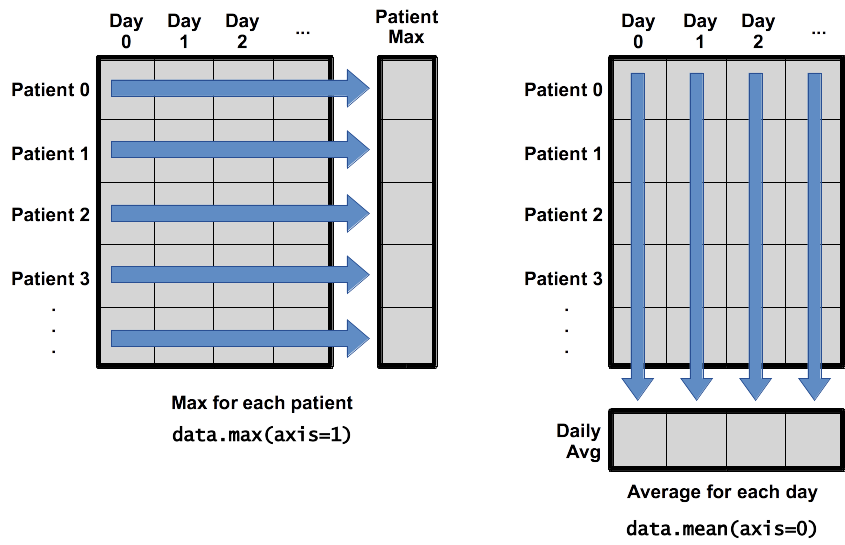
Operations Across Axes

To support this, most array methods allow us to specify the axis we want to work on. If we ask for the average across axis 0 (rows in our 2D example), we get:

print(data.mean(axis=0))

[  0.           0.45         1.11666667   1.75         2.43333333   3.15
   3.8          3.88333333   5.23333333   5.51666667   5.95         5.9
   8.35         7.73333333   8.36666667   9.5          9.58333333
  10.63333333  11.56666667  12.35        13.25        11.96666667
  11.03333333  10.16666667  10.           8.66666667   9.15         7.25
   7.33333333   6.58333333   6.06666667   5.95         5.11666667   3.6
   3.3          3.56666667   2.48333333   1.5          1.13333333
   0.56666667]

As a quick check, we can ask this array what its shape is:

print(data.mean(axis=0).shape)

(40,)

The expression (40,) tells us we have an N×1 vector, so this is the average inflammation per day for all patients. If we average across axis 1 (columns in our 2D example), we get:

print(data.mean(axis=1))

[ 5.45   5.425  6.1    5.9    5.55   6.225  5.975  6.65   6.625  6.525
  6.775  5.8    6.225  5.75   5.225  6.3    6.55   5.7    5.85   6.55
  5.775  5.825  6.175  6.1    5.8    6.425  6.05   6.025  6.175  6.55
  6.175  6.35   6.725  6.125  7.075  5.725  5.925  6.15   6.075  5.75
  5.975  5.725  6.3    5.9    6.75   5.925  7.225  6.15   5.95   6.275  5.7
  6.1    6.825  5.975  6.725  5.7    6.25   6.4    7.05   5.9  ]

which is the average inflammation per patient across all days.

The mathematician Richard Hamming once said, “The purpose of computing is insight, not numbers,” and the best way to develop insight is often to visualize data. Visualization deserves an entire lecture (or course) of its own, but we can explore a few features of Python’s matplotlib library here. While there is no “official” plotting library, this package is the de facto standard. First, we will import the pyplot module from matplotlib and use two of its functions to create and display a heat map of our data:

import matplotlib.pyplot
image  = matplotlib.pyplot.imshow(data)
matplotlib.pyplot.show()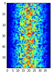

Heatmap of the Data

Blue regions in this heat map are low values, while red shows high values. As we can see, inflammation rises and falls over a 40-day period.

Let’s take a look at the average inflammation over time:

ave_inflammation = data.mean(axis=0)
ave_plot = matplotlib.pyplot.plot(ave_inflammation)
matplotlib.pyplot.show()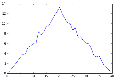

Average Inflammation Over Time

Here, we have put the average per day across all patients in the variable ave_inflammation, then asked matplotlib.pyplot to create and display a line graph of those values. The result is roughly a linear rise and fall, which is suspicious: based on other studies, we expect a sharper rise and slower fall. Let’s have a look at two other statistics:

max_plot = matplotlib.pyplot.plot(data.max(axis=0))
matplotlib.pyplot.show()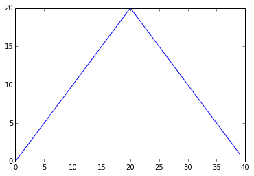

Maximum Value Along The First Axis

min_plot = matplotlib.pyplot.plot(data.min(axis=0))
matplotlib.pyplot.show()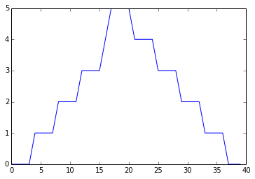

Minimum Value Along The First Axis

The maximum value rises and falls perfectly smoothly, while the minimum seems to be a step function. Neither result seems particularly likely, so either there’s a mistake in our calculations or something is wrong with our data. This insight would have been difficult to reach by examining the data without visualization tools.

You can group similar plots in a single figure using subplots. This script below uses a number of new commands. The function matplotlib.pyplot.figure() creates a space into which we will place all of our plots. The parameter figsize tells Python how big to make this space. Each subplot is placed into the figure using its add_subplot method. The add_subplot method takes 3 parameters. The first denotes how many total rows of subplots there are, the second parameter refers to the total number of subplot columns, and the final parameter denotes which subplot your variable is referencing (left-to-right, top-to-bottom). Each subplot is stored in a different variable (axes1, axes2, axes3). Once a subplot is created, the axes can be titled using the set_xlabel() command (or set_ylabel()). Here are our three plots side by side:

import numpy
import matplotlib.pyplot

data = numpy.loadtxt(fname='inflammation-01.csv', delimiter=',')

fig = matplotlib.pyplot.figure(figsize=(10.0, 3.0))

axes1 = fig.add_subplot(1, 3, 1)
axes2 = fig.add_subplot(1, 3, 2)
axes3 = fig.add_subplot(1, 3, 3)

axes1.set_ylabel('average')
axes1.plot(data.mean(axis=0))

axes2.set_ylabel('max')
axes2.plot(data.max(axis=0))

axes3.set_ylabel('min')
axes3.plot(data.min(axis=0))

fig.tight_layout()

matplotlib.pyplot.show()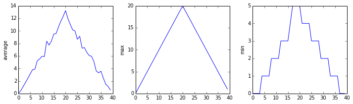

The Previous Plots as Subplots

The call to loadtxt reads our data, and the rest of the program tells the plotting library how large we want the figure to be, that we’re creating three subplots, what to draw for each one, and that we want a tight layout. (Perversely, if we leave out that call to fig.tight_layout(), the graphs will actually be squeezed together more closely.)

mass = 47.5
age = 122
mass = mass * 2.0
age = age - 20

first, second = 'Grace', 'Hopper'
third, fourth = second, first
print(third, fourth)

element = 'oxygen'
print('first three characters:', element[0:3])
print('last three characters:', element[3:6])

first three characters: oxy
last three characters: gen